
DRAGONDOCK
Autonomous spacecraft rendezvous and docking simulation with integrated GNC for a Dragon-to-ISS proximity operations scenario.
Project Overview
DRAGONDOCK simulates the complete GNC pipeline for a SpaceX Dragon capsule autonomously approaching and docking with the ISS — from 100 km separation down to sub-meter accuracy. Developed for Stanford's AA279D (Spacecraft Formation-Flying and Rendezvous, Prof. Simone D'Amico), the simulation operates in J2-perturbed LEO and progresses from foundational orbital mechanics through a fully integrated navigation-control closed loop.
Technical Architecture
Dynamics & Propagation
The deputy state is represented as quasi-non-singular relative orbital elements (QNSROE) — chosen because the ISS's near-circular orbit makes classical elements singular. The chief is propagated in ECI with J2-perturbed two-body dynamics; the deputy uses D'Amico's analytical J2 STM, which captures secular J2 drift without numerical integration. We also implemented HCW and Yamanaka-Ankersen propagators and validated all three against a full nonlinear truth to quantify where each linearization breaks down.
Navigation System
A 12-state Unscented Kalman Filter jointly estimates chief and deputy states. The chief carries GPS (cm-level noise); the deputy only has lidar (range at close proximity) and camera (bearing angles, no range). We chose UKF over EKF because the measurement model — chaining ROE→OE→ECI→range/angles — involves highly nonlinear transforms where analytical Jacobians would be fragile. The filter was validated through 3σ bound consistency checks.
Control Design
A Lyapunov-based continuous controller drives the deputy toward the target state. The control law u = -pinv(B)·(A·δα + P·error) combines feedforward cancellation of natural orbital drift with proportional error feedback. The P matrix concentrates thrust at fuel-optimal orbital positions using cosine weighting — only burning when the geometry is favorable. Stability is provable under ideal state knowledge (V̇ ≤ 0); under realistic estimation noise, convergence was validated through Monte Carlo simulation. Total delta-v: 43 m/s over ~15 orbits.
Results
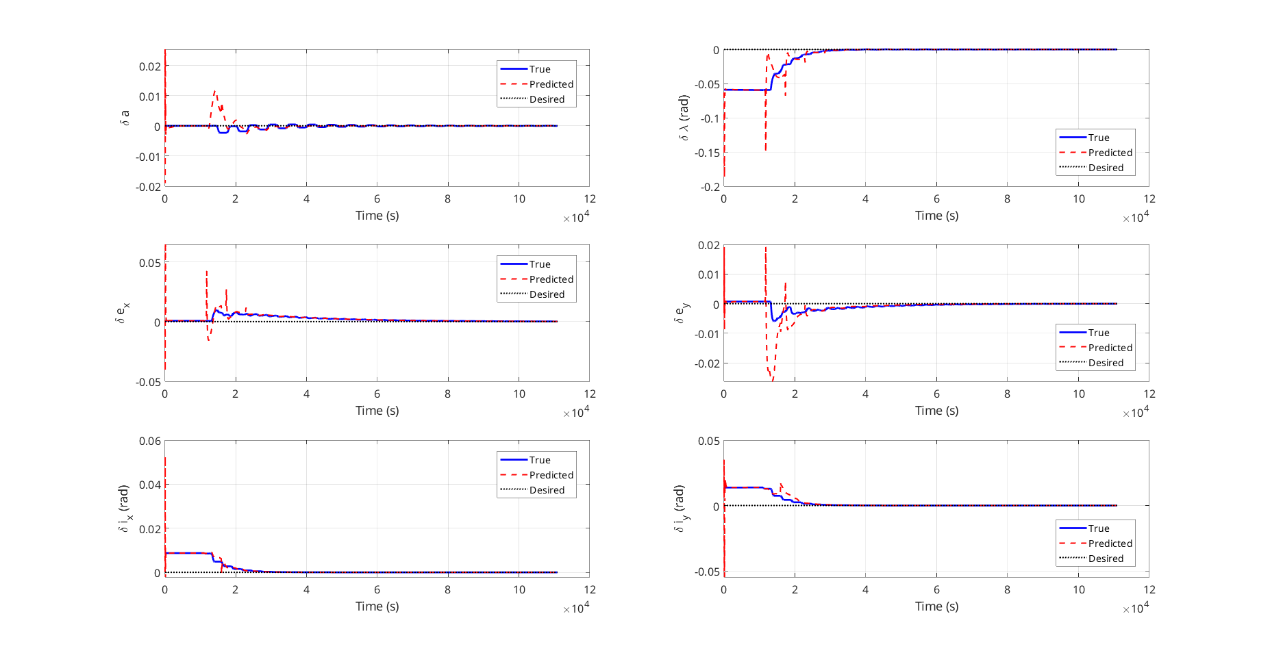
QNSROE Convergence — Deputy orbital elements converging to target
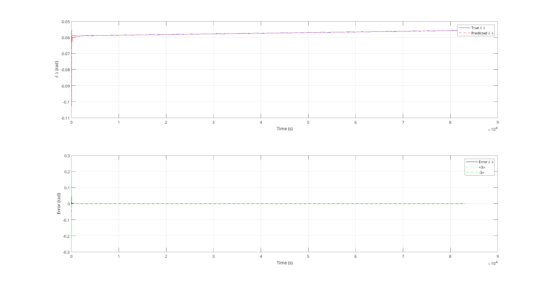
UKF Estimation Error — State errors with ±3σ bounds
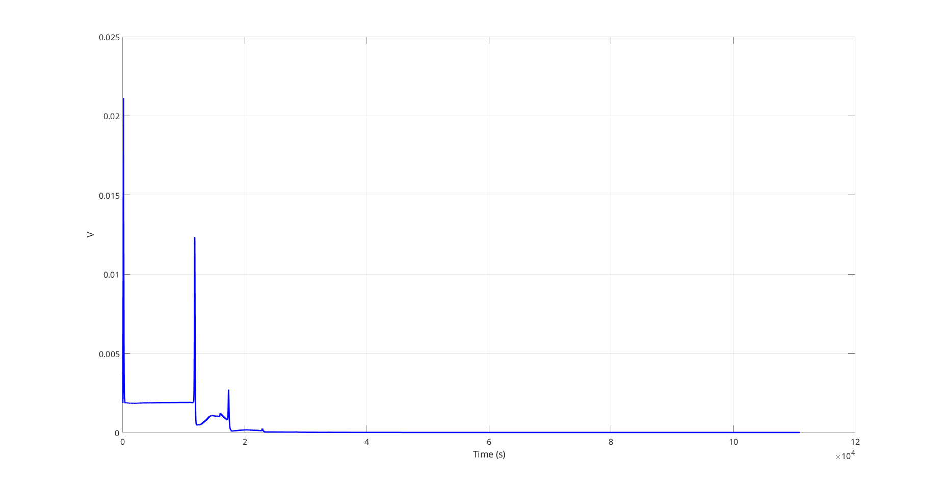
Lyapunov Function — Monotonic decrease proving stability
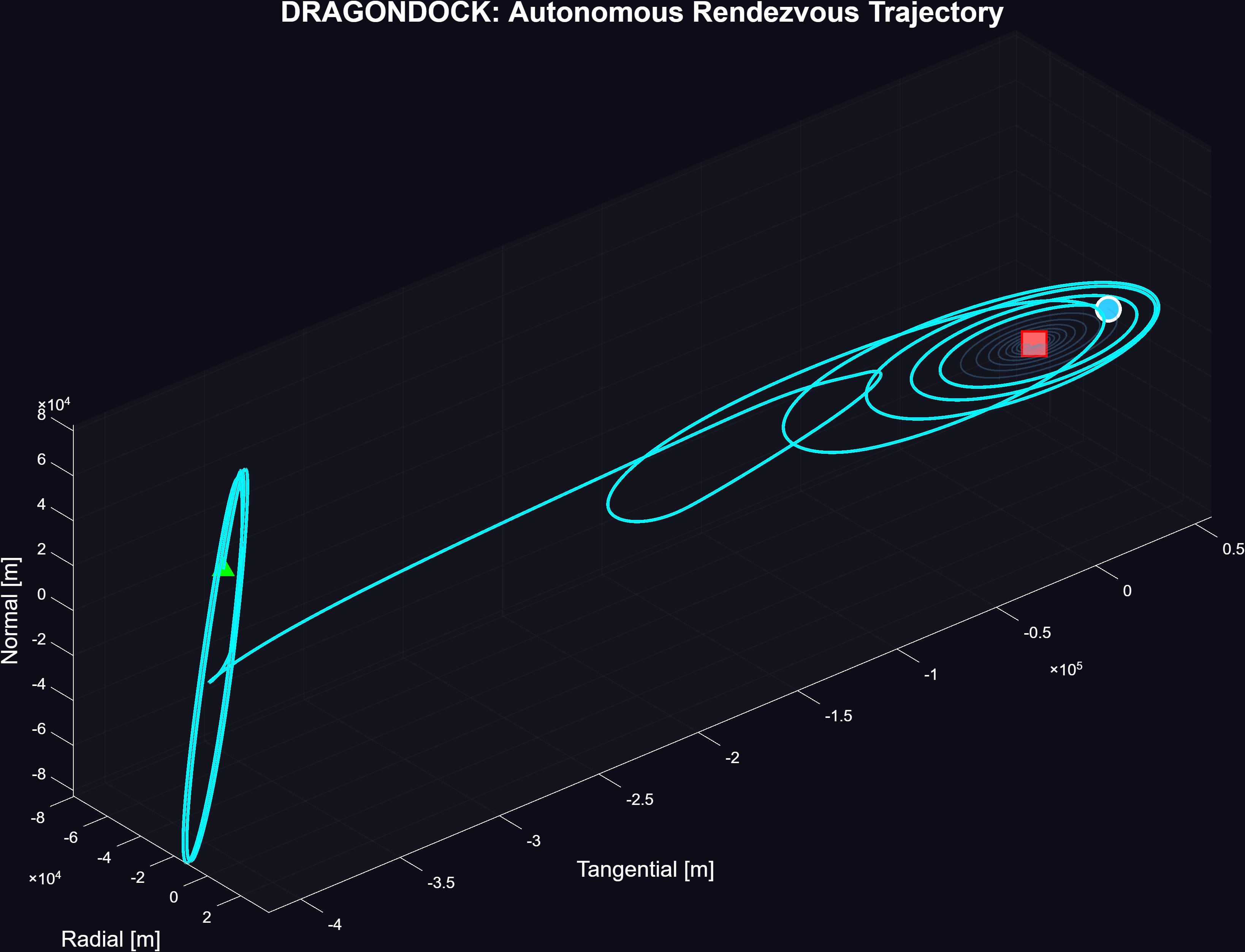
RTN Trajectory — Relative motion in chief frame
Simulation Video — Animated rendezvous sequence
Technical Challenges
Dynamics Model Selection & Validation
We implemented four propagators — two-body Keplerian, J2-perturbed nonlinear, HCW linearized relative motion, and Yamanaka-Ankersen for eccentric orbits. We ran each against the J2 nonlinear truth to quantify where they diverge and why. HCW drifts because it assumes circular orbits and no J2. Yamanaka-Ankersen handles eccentricity but ignores J2. This comparison drove the decision to use the J2-perturbed STM for both control and estimation — the accuracy penalty of cheaper models was too large over 20 orbits.
Mean vs Osculating Element Consistency
The controller operates on mean QNSROE but truth dynamics produce osculating elements. The J2 short-period oscillations appear as phantom errors the controller tries to correct, wasting fuel. The solution was ensuring the UKF outputs mean element estimates — not osculating — by applying mean-osculating conversion at the measurement update step, so the controller receives the representation it was designed for.
Sensor Fusion Across Measurement Types
The chief has GPS (cm-level noise, absolute position). The deputy only has lidar (precise range at close proximity) and camera (bearing angles, no range). The UKF fuses these by using different measurement models for each sensor and adjusting the measurement noise covariance R accordingly. The key challenge was sensor handoff — when lidar becomes available at close range, the filter's confidence bounds must transition smoothly. We tuned the process noise Q to prevent overconfidence during camera-only phases, so the filter doesn't overcorrect when lidar first comes online.
Closed-Loop Stability With Estimation Error
The Lyapunov stability proof assumes perfect state knowledge — V̇ ≤ 0 only holds if you know δα exactly. In the closed-loop system, the controller receives the UKF's noisy estimate instead, so that guarantee breaks. We addressed this by selecting conservative controller gains (lower K in u = -Bc†Kδα) that tolerate estimation noise without overreacting, and validated convergence through Monte Carlo runs across randomized initial conditions and noise realizations. Every run converged with sub-meter accuracy.